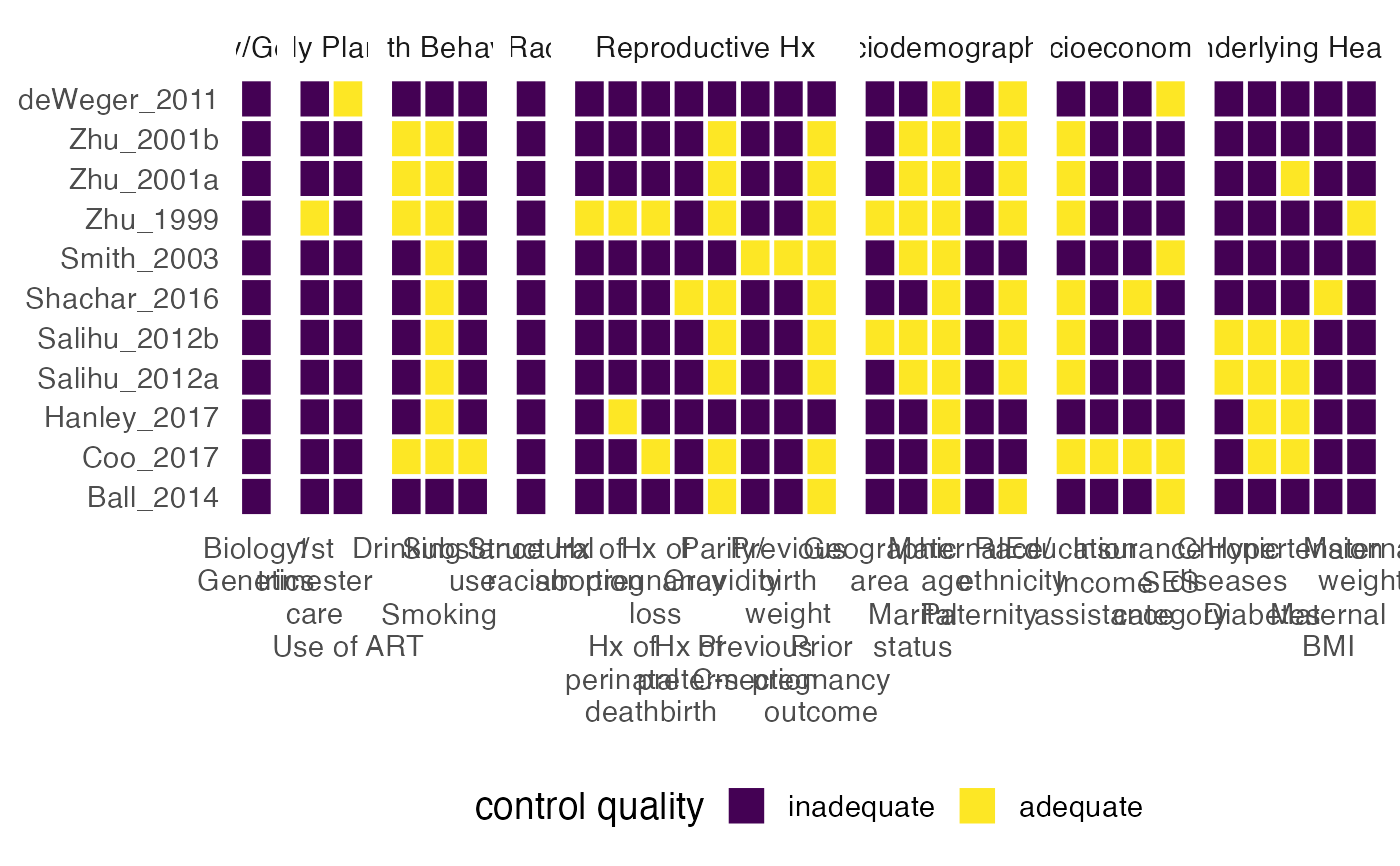
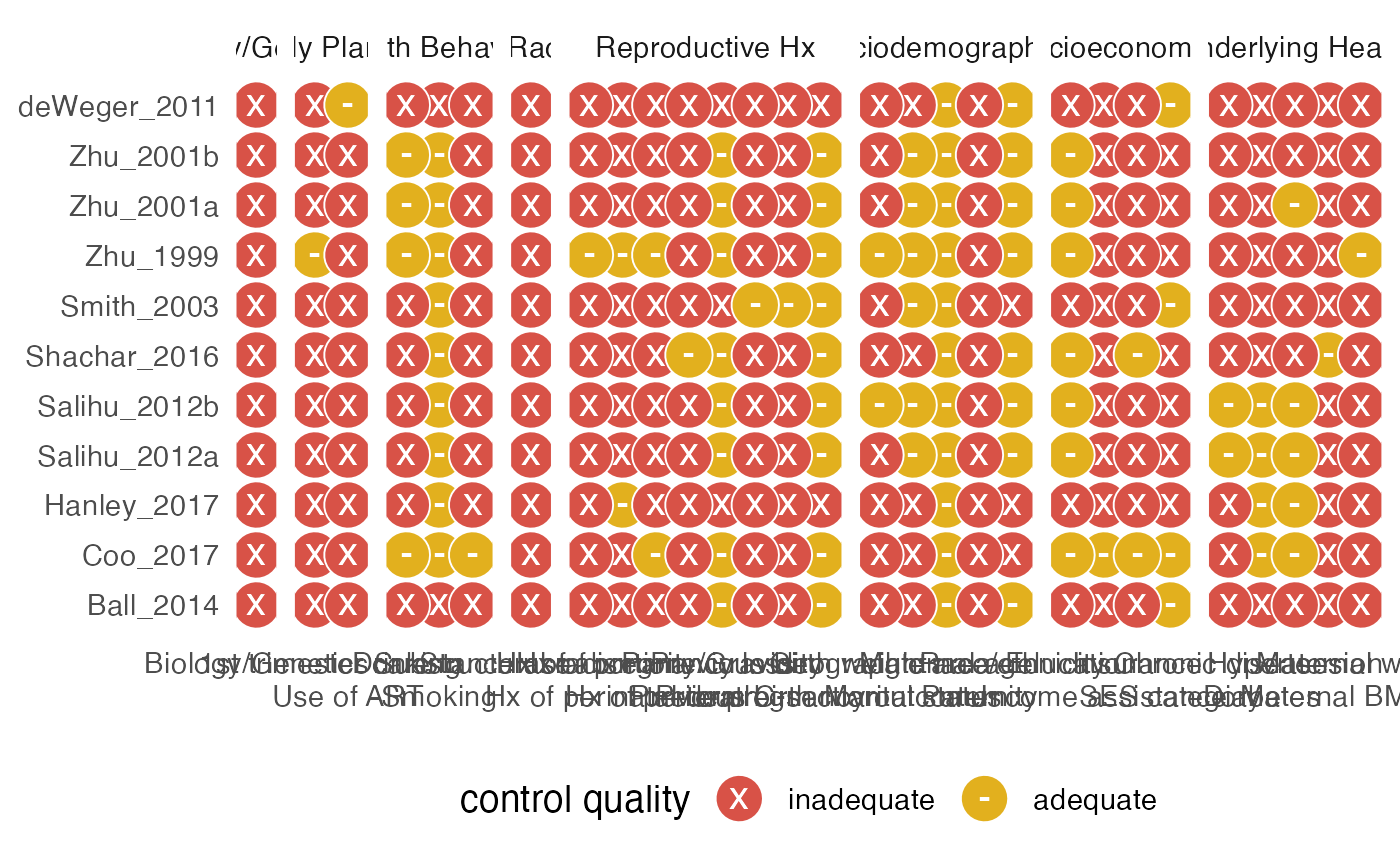
mc_heatmap() and mc_trafficlight() visualize the results of
metaconfoundr(), summarizing the quality of confounder control in each
study.
mc_heatmap(
  .df,
  legend_title = "control quality",
  sort = FALSE,
  by_group = FALSE,
  score = c("adequate", "sum", "controlled"),
  non_confounders = FALSE
)

mc_trafficlight(
  .df,
  size = 8,
  legend_title = "control quality",
  sort = FALSE,
  by_group = FALSE,
  score = c("adequate", "sum", "controlled"),
  non_confounders = FALSE
)
Arguments
- .df
A data frame, usually the result of
metaconfoundr()- legend_title
The legend title
- sort
Logical. Sort by confounder score? Calculated by
score_control()- by_group
Logical. If sorted, sort within domain?
- score
The approach used to calculate the score.
adequatetests if the study controlled at a strictly adequate level.sumtreatscontrol_qualityas an ordinal integer, summing it's values such that a higher score has better control overall.controlledtests if any control, includingsome concernscontrol, is present.- non_confounders
Logical. Include non-confounders? Default is
FALSE.- size
The size of the points in the traffic light plot
Value
a ggplot
See also
Other plots:
facet_constructs(),
geom_cochrane(),
scale_fill_cochrane(),
theme_mc()
Examples
ipi %>%
  metaconfoundr() %>%
  dplyr::mutate(variable = stringr::str_wrap(variable, 10)) %>%
  mc_heatmap() +
  theme_mc() +
  facet_constructs() +
  ggplot2::guides(x = ggplot2::guide_axis(n.dodge = 2))


ipi %>%
  metaconfoundr() %>%
  mc_trafficlight() +
  geom_cochrane() +
  facet_constructs() +
  scale_fill_cochrane() +
  theme_mc() +
  ggplot2::guides(x = ggplot2::guide_axis(n.dodge = 2))
